[Sticky post:  This post will remain at the top of the main page until 04/18/18.  Scroll down to see the latest CHM 110 and CHM 111 notes or announcements.]

If you’re in the Wednesday morning or Tuesday afternoon CHM 110 labs (sections 1 or 2), you’re probably working on your report for experiment 7.  To finish your report for Experiment 7 (the cobalt chloride spectrometry lab), you’ll need to do two main things.

1. Plot the data from test tubes 1-7 to find the Beer’s Law constant, k.
2. Use Beer’s Law to determine the concentration of the unknown.

Click the link below for some help making the Beer’s Law plot and calculating the concentration of your unknown.

Making the plot

How do you do these things?  First, you’ll need to calculate the concentrations of the known CoCl₂ solutions.  You can do this since you made each one by mixing known amounts of 0.150 M CoCl₂ stock solution and water.  Other than Tube #1, which is simply the 0.150 M CoCl₂, each other tube was made by dilution, and you can calculate the new CoCl₂ concentration using the dilution equation

M₁V₁ = M₂V₂

… where:

• M₁ = the concentration of the original solution
• V₁ = the volume of the original solution
• M₂ = the concentration of the new (diluted) solution
• V₂ = the total volume of the new (diluted) solution

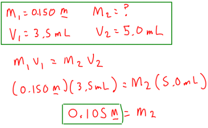
I’ll use Tube #3 as an example.  Tube #3 contains 3.5 mL of 0.150 M CoCl₂ mixed with 1.5 mL of distilled water.  This makes a new solution with a total volume of 5.0 mL (3.5 + 1.5).

Sample calculation for the concentration of Tube #3

So, the concentration of CoCl₂ in Tube #3 is 0.105 M (0.11 M rounded to two significant figures.  The table with the information you used to prepare each solution is on page 138 in the lab manual.

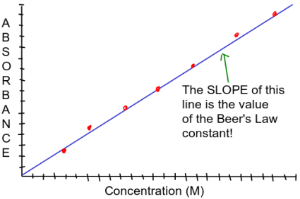
Once you calculate the concentration of CoCl₂ in Tubes 1-7, then plot the absorbance data using a spreadsheet program on your computer or in one of the computer labs at Tech.  Plot absorbance on the vertical (y) axis and concentration on the horizontal (x) axis.  Make sure the data is linear – it should look something like this:

Sample Beer’s Law plot

You will need to calculate the slope of the line.  Since you’re using a spreadsheet to make your plot, use the spreadsheet to calculate the slope of the line: click on the data and “add trend line”.

The slope of the line is equal to the Beer’s Law constant, k.

The unknown

If you know the Beer’s Law constant, you can calculate the concentration of the unknown by using the simplified form of Beer’s Law.

A = kc

…where

• A = absorbance
• k = Beer’s Law constant
• c = molar concentration of the diluted unknown (this will be M₂ in your next calculation)